 汉语
汉语
 English
 Français
 Deutsch


Direct Answer: PID tuning optimizes liquid flow controller performance by adjusting Proportional, Integral, and Derivative control parameters. These changes help the system achieve response times as fast as 0.3 seconds to within ±1 % of set-point. By configuring bias/offset settings for initial valve positioning and fine-tuning PID zones for different flow rates, processing time is reduced, throughput increases, and liquid waste is minimized in semiconductor manufacturing applications.
Table of Contents
- What is PID tuning and why does it matter for liquid flow controllers?
- How do different liquid flow measurement technologies impact response times?
- What are the key components of effective PID tuning?
- How do PID zones optimize performance across multiple flow rates?
- What role does bias/offset play in fast response times?
- How can you implement dynamic bias/offset for machine learning optimization?
- What is the step-by-step process for tuning PID values?
- Ready to optimize your liquid flow control system?
- Conclusion: Achieving sub-second response times through proper PID tuning
1. What is PID tuning and why does it matter for liquid flow controllers?
PID tuning is the process of configuring Proportional (P), Integral (I), and Derivative (D) control parameters to optimize the real-time feedback control loop in liquid flow controllers. This tuning directly impacts both the speed and accuracy of achieving and maintaining your set-point flow rate.
The need for fast and precise tuning is critical in semiconductor processes like short-pulse Chemical Vapor Deposition (CVD) or Atomic Layer Deposition (ALD). In these applications, a delay in stabilization — even by a few seconds — negatively impacts throughput and increases waste.
Key benefits of optimized PID tuning include:
- Increased throughput, allowing more wafers to be processed per hour
- Reduced waste by decreasing time spent sending vapor to diverter lines
- Improved process control through tighter flow regulation and better Statistical Process Control (SPC)
- Enhanced equipment uptime thanks to less maintenance on pumps and remediation systems
2. How do different liquid flow measurement technologies impact response times?
The choice of measurement technology directly affects how quickly your PID loop responds and stabilizes liquid flow. Consider the following options:
Thermal Flow Measurement Limitations
Thermal flow meters are cost-effective but have speed limitations in liquid measurement:
- Response times typically are three seconds or longer
- Flow changes are detected more slowly
- Control loop adjustments are less precise
- Each liquid requires specific calibration
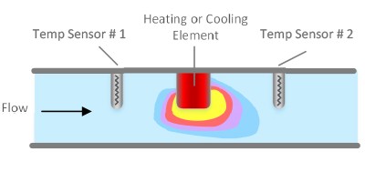
Image 1: Thermal flow sensor illustration - In this method, the liquid is heated (or cooled) and the speed at which the liquid cools (or heats) can be calibrated to liquid flow rates.
Coriolis Flow Measurement Challenges
Coriolis meters offer high accuracy but present speed challenges due to their measurement principle:
- Large number of deflection measurements needed for accuracy
- Sensitivity to vibration and environmental conditions
- Complex tube geometries prone to bubble formation
- Higher pressure drops that can affect system performance
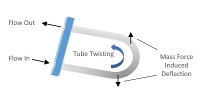
Image 2: Illustration of Coriolis effect in curved tube which causes deflection and twisting. In practice, a vibration is often induced on the curved tube, and the frequency of the vibration as detected by optoelectrical sensors is related to mass flow rate.
Differential Pressure: The Speed Advantage
Differential pressure liquid flow controllers excel in speed-critical applications because pressure changes can be sensed significantly faster than temperature changes or statistical deflection measurements:
- Measurement frequency of 10ms intervals
- Faster control loops enabling tighter flow control
- Straightforward fluid mechanics allowing calculation-based liquid switching
- Simplified PID tuning due to rapid sensor response
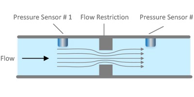
Image 3: Illustration of a type of differential pressure flow sensor - Differential pressure liquid flow meters are based on the phenomenon that pressure drop across a flow restriction is a function of liquid flow rate.
3. What are the key components of effective PID tuning?
Understanding each PID component helps optimize controller performance for specific applications and flow rates.
Proportional (P) Control
The Proportional component acts as a multiplier of the difference between set-point and measured value. Key characteristics include:
- Function: Amplifies the error signal to drive faster corrections
- Effect: Higher P values increase response speed but can cause oscillation
- Optimization: Start with moderate values and increase gradually while monitoring for instability
Integral (I) Control
The Integral component addresses accumulated error over time, providing steady-state accuracy:
- Function: Sums error differences over time to eliminate offset
- Effect: Higher I values provide faster adjustment to persistent errors
- Optimization: Often the primary parameter to adjust for faster response, with values up to 15 being common
Derivative (D) Control
The Derivative component responds to the rate of change in measured values:
- Function: Anticipates future error based on current rate of change
- Effect: Can speed response but may cause system instability
- Optimization: Use sparingly and only when overshoot must be prevented
4. How do PID zones optimize performance across multiple flow rates?
If your process has multiple liquid flow setpoints – for example 1g/min, 5g/min, 15g/min and 30g/min; for completely optimized response times you would set unique PID parameters for each of these set-points using ‘zones’. PID values are typically loaded into a device using a ‘recipe table’ (Table 1). In a recipe table, there are ‘zones’ of control. For optimized response, it is best to set the PID parameters specific to the set-point. In the recipe table, a ‘zone’ is defined by the top % F.S. (Full Scale) value (see Table 1 Column 2 - Threshold).
The zone includes all flow rates less than the Threshold value and everything above the Threshold value of the previous zone. For example, if the Zone 0 Threshold value is 5 (5% F.S.), then for a 30g/min full scale unit the first zone would include set-points from 0 – 1.5g/min. If the second zone had a threshold value of 10% F.S., then the second zone would run from 1.51 – 3.00 g/min.
In the Turbo™ 2950 LFC, there are 8 zones that can be configured. These zones do not need to be spread evenly across the full scale. Ideally, you would have one zone for each unique set-point if you are looking for optimized response.
| Zone | Threshold (% F.S.) |
Example values (g/min) |
Bias/ Offset (V) |
Example Valve Position |
Bias/ Offset Time (ms) |
|---|---|---|---|---|---|
| 0 | 5 | 0-1.50 | 2 | 98% open | 200 |
| 1 | 10 | 1.51-3.00 | 2 | 98% open | 200 |
| 2 | 15 | 3.01-4.50 | 2 | 98% open | 200 |
| 3 | 20 | 4.51-6.00 | 2 | 98% open | 200 |
| 4 | 30 | 6.01-9.00 | 70 | 30% open | 200 |
| 5 | 70 | 9.01-21.00 | 60 | 40% open | 200 |
| 6 | 75 | 21.01-22.50 | 40 | 60% open | 200 |
| 7 | 90 | 22.51-30.00 | 90 | 10% open | 200 |
In lower flow zones, prioritize higher I values for sensitivity. In medium zones, balance P and I. At higher flow rates, more conservative settings reduce overshoot.
5. What role does bias/offset play in fast response times?
The bias/offset options determine how quickly the LFC initially reaches the set-point. Essentially, these options can allow the user to control the shape and speed of the initial flow response.
If bias/offset is used, when a set-point is received, the flow controller tells the control valve to move to a pre-determined position for a fixed amount of time (typically milliseconds). Valve position is determined by voltage (Column 4 in Table 1), and Bias/Offset Time (Column 6 in Table 1) is the amount of time the controller will hold at this fixed voltage before engaging the PID control loop. In the 2950 LFC, ~100 - 120V is fully closed and 0 V is fully open. Columns 4 and 5 provide a rough guide of how voltage relates to valve position (not absolute – example only; application/hardware specific).
Recipe Bias/Offset Method
 Aggressive approach: Opens valve to ~98% for rapid flow establishment
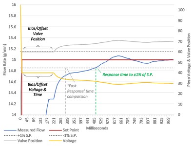
On one end of the spectrum, bias/offset can be used to ‘jumpstart’ the flow; by opening the valve ~100% for a short period of time to quickly establish flow (Figure 1), before then moving into the PID control loop. In this case, a low bias/offset voltage would be applied. Doing this can significantly improve the time to set-point, but also likely results in some ‘overshoot’ as well (particularly if the bias/offset time is too long).
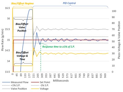
Figure 1 is an illustration of a flow pulse (flow set-point event: start to finish). The red line is the flow set point signal, the blue line is the measured flow rate (both left axis). The grey line is the valve position and the yellow line is the piezo voltage (both the right axis). The piezo voltage to valve position is very application specific and is just an example for discussion purposes. The left part of the graph is the bias/offset region. Shown is the bias voltage and valve position and the time they stay at these set-points (bias/offset time). After the bias/offset regime, PID control takes over (middle/right of the graph). In this example, the bias/offset is set to overdrive the liquid flow to bring the flow to set-point quickly; similar to how the Recipe Bias/Offset voltage is set in Zones 0,1,2 & 3 in Table 1.
 Conservative approach: Uses moderate opening to prevent overshoot
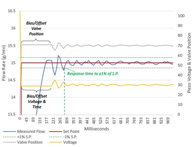
On the other end of the spectrum, bias/offset could be used to ensure the valve does not open too far initially – to prevent ANY overshoot. In this case a bias/offset voltage of 80-100V would be used.
Figure 2 is an illustration of a bias/offset and PID set to reduce/eliminate overshoot. In this case, bias/offset voltage is set high – corresponding to a more closed valve position, similar to how the Recipe Bias/Offset voltage is set in Zone 7 in Table 1. This ensures the initial flow set-point will not overshoot. Additionally, PID values in this example are set to make small changes to flow errors; again, to reduce/prevent overshoot. Note the response time is slower versus Figure 1 Bias/Offset Voltage Illustration: Overdrive - Fast Response.
 Balanced approach: Optimizes between speed and stability
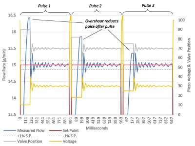
Bias/Offset levels can be set aggressive - ‘jump-start’ shown in Figure 1; conservative - ‘creep-up’ approach shown in Figure 2, or somewhere in between - as illustrated by Figure 3 and in the recipe bias/offset voltage value examples in Table 1 zones 4, 5, & 6.
There are several different bias/offset methods to provide flexibility for application requirements and user preferences in the Turbo™ 2950 LFC.
Benefits of Proper Bias/Offset Configuration
- Faster initial response: Eliminates delay in valve movement
- Reduced overshoot: Prevents flow excursions beyond set-point
- Customizable response shape: Allows tailoring to specific process requirements
6. How can you implement dynamic bias/offset for machine learning optimization?
Dynamic bias/offset can be implemented as a lightweight, experience-based optimization layer that improves system response without modifying the core PID control loop. Instead of relying on a fixed, pre-defined starting valve position (as in a traditional recipe-based bias/offset method), the system continuously learns from previous set-point executions and adjusts the initial valve position accordingly.
From Static to Dynamic Optimization
In a conventional recipe bias/offset approach, each set-point is assigned a fixed valve position and duration. While predictable, this method cannot adapt to changing conditions such as fluid properties, environmental variations, or valve wear. Dynamic bias/offset overcomes this limitation by using historical performance data to refine the starting point for each new control cycle.
How Dynamic Bias/Offset Works
When dynamic bias/offset is enabled, the controller “learns” the optimal initial valve position for a given set-point based on prior pulses:
- Current Method (default): The system uses the valve position at the end (trailing edge) of the previous pulse as the starting point for the next one. This allows the controller to progressively reduce overshoot and improve accuracy with each repetition.
 Alternate Method: The system determines the starting valve position based on conditions observed at the beginning (leading edge) of the previous pulse, once a defined stability threshold and time are met. This approach is useful in scenarios with very short pulses or long idle periods, where end-of-pulse conditions may not reflect the next starting state.
Figure 4 is an illustration of dynamic bias. From pulse 1 to 3, the measured flow (blue line) overshoot lessons, the valve position (grey) and piezo voltage (yellow) change to become closer to the correct starting point for that set-point. Note: only the bias/offset regime is changed. The PID control region is not changed.
Key Implementation Principles
- Learning is iterative: Each repeated set-point refines the starting valve position, improving performance over time.
- PID remains unchanged: Only the initial bias/offset (valve position) is adjusted, ensuring system stability and predictability.
- Adaptive to real conditions: The system accounts for drift caused by temperature changes, environmental factors, and component aging.
- Faster stabilization: By starting closer to the optimal operating point, the system reduces overshoot and achieves target flow more quickly.
When to Use Dynamic Bias/Offset
Dynamic bias/offset is most effective in applications with repeated or cyclical set-points, where the system can continuously learn and optimize. The Current method is typically preferred for most applications due to its strong response time performance, while the Alternate method is beneficial in edge cases involving transient or thermally sensitive conditions.
 By implementing dynamic bias/offset, you introduce a practical form of machine learning into your control strategy—one that enhances response time, improves repeatability, and adapts to real-world process variability, all while maintaining the robustness of established PID control.
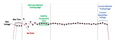
Figure 5 is an illustration of how bias/offset voltage is calculated when using either Dynamic Bias/Offset Current or Dynamic Bias/Offset Alternate. In Dynamic Bias/Offset Current method, the bias/offset voltage for the next pulse is determined by the last few points of the previous pulse setpoint. In Dynamic Bias/Offset Alternate method, the bias/offset voltage for the next pulse is determined on the leading edge of the pulse after a user defined stability threshold and stability interval is satisfied.
7. What is the step-by-step process for tuning PID values?
A systematic approach builds consistency and reliability into PID tuning. Use this structured process:
Step 1: Initial Setup and Reset
- Set flow rate to zero; close control valve
- Reset PID calculations
- Begin with baseline values (P = 1, I = 1, D = 0)
- Record current performance
Step 2: Optimize Integral (I) Parameter
- Use I as the primary tuning parameter
- Increase gradually — values up to 15 are common
- Watch for oscillation or instability; reduce if present
- Note the optimal setting
Step 3: Adjust Proportional (P) if Needed
- If target response is not achieved with I, increase P slowly
- Monitor for set-point oscillation
- Rely less on P if a dynamic bias/offset method is in use
Step 4: Consider Derivative (D) Only if Required
- Employ D only to address overshoot
- Increase in small increments
- Monitor stability carefully
Step 5: Validation and Documentation
- Conduct multiple test cycles at tuned settings
- Verify repeatability across trials
- Document PID values for each zone
Common Troubleshooting Issues
Flow oscillation, slow response, and overshoot are the most common problems. Solutions include:
- For oscillation: Lower P and I values
- For slow response: Gradually increase I, then P
- For overshoot: Use conservative bias/offset or add a small D component
8. Ready to optimize your liquid flow control system?
 Achieving sub-second response times hinges on fast hardware and agile control algorithms. The TSI MSP Turbo™ 2950 Liquid Flow Controller uses differential pressure sensing and advanced PID tuning to help you reach response times as fast as 0.3 seconds.
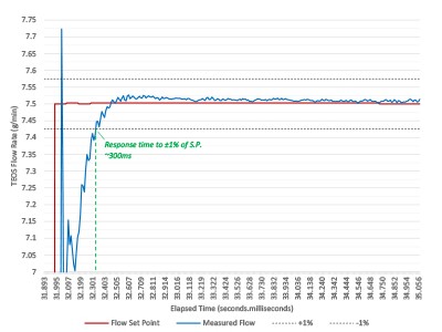
Figure 6 shows the Turbo™ 2950-30 LFC Response Time - By choosing a fast response LFC and by optimizing PID tuning, response times ≤ ±0.3s to 1% of set-point can readily be achieved.
Key features supporting fast PID tuning:
- Eleven-millisecond measurement intervals for rapid updates
- Eight configurable PID zones for flow-rate-specific tuning
- Dynamic bias/offset learning to drive continuous performance gains
- EtherCAT and RS485 communication for integration flexibility
- Field-configurable software to simplify PID parameter adjustments
Take Action Today
Boost your process throughput — connect with our flow control specialists to explore how PID tuning with the MSP Turbo™ 2950 can help you achieve significant production improvements.
More About the MSP Turbo™ Liquid Flow Controllers
9. Conclusion: Achieving sub-second response times through proper PID tuning
Optimizing liquid flow controller performance with proper PID tuning routinely reduces response times from three or more seconds to as little as 0.3 seconds. This advance delivers not only higher throughput but also reduced liquid waste and enhanced stability — vital for modern CVD and ALD processes. Select high-speed, differential pressure-based controllers, configure PID zones and bias/offset strategies effectively, and follow structured tuning procedures to reach optimal results with advanced equipment like the MSP Turbo™ 2950.
Sources & References
W. Chung, “Liquid Flowmeter Using Thermal Measurement; Design and Application”, Marquette University Thesis 2009.
W. Shannon, “9 Limitations of Thermal Mass Flowmeters (and How to Overcome Them)”, Flow Control, June 2017.
T. Wang, R. Baker, “Coriolis flowmeters: a review of developments over the past 20 years, and an assessment of the state of the art and likely future directions, Flow Measurement and Instrumentation, December 2014, 40,99-123.
P. Bruschi, M. Piotti, G. Barillaro, “Effects of gas type on the sensitivity and transition pressure of integrated thermal flow sensors,” Sensors and Actuators, 182-187, 2006.
J. H. Ahn, K.T. Kang, K. H. Ahn, “Development and Evaluation of Differential Pressure Type Mass Flow Controller for Semiconductor Fabrication Processing,” Journal of the Semiconductor & Display Equipment Technology, 7(4),29-34, 2008.